(著)山拓
気になったのでPythonで実装しました。まあ、微分方程式解けばよいのですが。
1-コンパートメントモデル
モデル

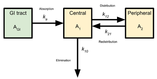
(図引用)http://www.turkupetcentre.net/petanalysis/pk_2cm.html
指数関数的に吸収されて指数関数的に排出される単純なモデル。式は次のようになる。
\begin{align*} \frac{dA(t)}{dt}&=-k_{a} A(t)\\ \frac{d C_{1}(t)}{d t} &=k_{a} A(t)-k_{10} C_{1}(t) \end{align*}
実装
実装はEuler法を使って適当にした。描画にjapanize-matplotlib(Qiita)を用いた。
import numpy as np
import matplotlib.pyplot as plt
import japanize_matplotlib
dt = 0.025 # hour
ka = 1
k10 = 0.2
T = 48 # hour
nt = round(T/dt) #Time steps
def one_compartment_model(c1, A, adm):
A = A*(1-ka*dt) + adm
c1 = A*ka*dt + c1*(1-k10*dt)
return c1, A
# once administration
c1 = 0; A = 0; # initial
c1_once = []
for i in range(nt):
if i == 0:
adm = 7 #administration
else:
adm = 0
c1, A = one_compartment_model(c1, A, adm)
c1_once.append(c1)
# Repeated administration
c1 = 0; A = 0; # initial
c1_repeated = []
step = 150
for i in range(nt):
if i % step== 0:
adm = 7 #administration
else:
adm = 0
c1, A = one_compartment_model(c1, A, adm)
c1_repeated.append(c1)
# Plot
t = np.arange(nt)*dt
plt.figure(figsize=(6, 3))
plt.subplot(1,2,1)
plt.plot(t[:int(nt/2)], np.array(c1_once)[:int(nt/2)])
plt.xlabel('時間')
plt.ylabel('血中濃度(C)')
plt.subplot(1,2,2)
plt.plot(t[:int(nt/2)], np.log(np.array(c1_once)[:int(nt/2)]))
plt.xlabel('時間')
plt.ylabel('log濃度')
plt.tight_layout()
plt.savefig('one_comp_model_1.png')
#plt.show()
plt.figure(figsize=(6, 3))
plt.plot(t, np.array(c1_once),linestyle="dashed", label="単回投与")
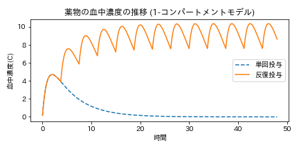
plt.plot(t, np.array(c1_repeated), label="反復投与")
plt.title('薬物の血中濃度の推移 (1コンパートメントモデル)')
plt.xlabel('時間')
plt.ylabel('血中濃度(C)')
plt.legend()
plt.tight_layout()
plt.savefig('one_comp_model_2.png')
#plt.show()
結果
下図は時刻0に薬物を投与したときのコンパートメント内の薬物の濃度。右図は左図の対数を取ったもの。

下図は単回投与と反復投与の場合の比較。ある程度投与すると血中濃度は一定となる。
2-コンパートメントモデル
モデル
(図引用)http://www.turkupetcentre.net/petanalysis/pk_2cm.html
末梢へも薬物が拡散する場合のモデル。少し複雑。式は次のようになる。
\begin{align*} \frac{dA(t)}{dt}&=-k_{a} A(t)\\ \frac{d C_{1}(t)}{d t} &=k_{a} A(t)-\left(k_{10}+k_{12}\right) C_{1}(t)+k_{21} C_{2}(t) \\ \frac{d C_{2}(t)}{d t} &=k_{12} C_{1}(t)-k_{21}
C_{2}(t) \end{align*}
実装
import numpy as np
import matplotlib.pyplot as plt
import japanize_matplotlib

dt = 0.025 # hour
ka = 1
k10 = 0.2
k12 = 0.5
k21 = 0.1
T = 96 # hour
nt = round(T/dt) #Time steps

def two_compartment_model(c1, c2, A, adm):
    A = A*(1-ka*dt) + adm
    c1 = A*ka*dt + c1*(1-(k10+k12)*dt) + k21*c2*dt
    c2 = c2*(1-k21*dt) + k12*c1*dt
    return c1, c2, A

# once administration
c1 = 0; c2 = 0; A = 0; # initial
c1_once = []
for i in range(nt):
    if i == 0:
        adm = 0.3 #administration
    else:
        adm = 0
    c1, c2, A = two_compartment_model(c1, c2, A, adm)
    c1_once.append(c1)

# Repeated administration
c1 = 0; c2 = 0; A = 0; # initial
c1_repeated = []
step = 200
for i in range(nt):
    if i % step== 0:
        adm = 0.3 #administration
    else:
        adm = 0
    c1, c2, A = two_compartment_model(c1, c2, A, adm)
    c1_repeated.append(c1)

# Plot
t = np.arange(nt)*dt
plt.figure(figsize=(6, 3))
plt.subplot(1,2,1)
plt.plot(t[:int(nt/2)], np.array(c1_once)[:int(nt/2)])
plt.xlabel('時間')
plt.ylabel('血中濃度(C)')

plt.subplot(1,2,2)
plt.plot(t[:int(nt/2)], np.log(np.array(c1_once)[:int(nt/2)]))
plt.xlabel('時間')
plt.ylabel('log濃度')
plt.tight_layout()
plt.savefig('two_comp_model_1.png')
#plt.show()

plt.figure(figsize=(6, 3))
plt.plot(t, np.array(c1_once),linestyle="dashed", label="単回投与")
plt.plot(t, np.array(c1_repeated), label="反復投与")
plt.title('薬物の血中濃度の推移 (2-コンパートメントモデル)')
plt.xlabel('時間')
plt.ylabel('血中濃度(C)')
plt.legend()
plt.tight_layout()
plt.savefig('two_comp_model_2.png')
#plt.show()
結果
時刻0に薬物を投与したときの血中濃度。対数を取った場合、1-コンパートメントモデルと異なり、2相があることが分かる。

反復投与をした場合。1-コンパートメントモデルよりも定常となるのが遅い。

コメントをお書きください